05. Spatially Adapted Total Variation

Here a locally adapted regularization is shown. For this purpose the SATV algorithm was implemented. The application and the benefit are shown.

import numpy as np
import matplotlib.pyplot as plt
from matplotlib import image

from recon.utils.utils import psnr
from recon.interfaces import SATV, Smoothing

gt = image.imread("../data/phantom.png")
gt = gt/np.max(gt)
gt = gt

noise_sigma = 0.1*np.max(gt)

noisy_image = gt + np.random.normal(0, noise_sigma, size=gt.shape)

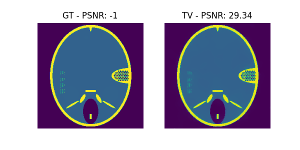
# TV smoothing small alpha
tv_smoothing = Smoothing(domain_shape=gt.shape, reg_mode='tv', alpha=1, lam=8)
u_tv = tv_smoothing.solve(data=noisy_image, max_iter=5000, tol=1e-4)


f = plt.figure(figsize=(6, 3))
f.add_subplot(1, 2, 1)
plt.axis('off')
plt.imshow(gt, vmin=0, vmax=np.max(gt))
plt.title("GT - PSNR: "+str(psnr(gt, gt)))
f.add_subplot(1, 2, 2)
plt.imshow(u_tv, vmin=0, vmax=np.max(gt))
plt.title("TV - PSNR: "+str(psnr(gt, u_tv)))
plt.axis('off')
plt.show(block=False)

Out:

Early stopping.

…

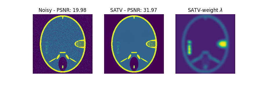
satv_obj = SATV(domain_shape=gt.shape,
                reg_mode='tv',
                lam=1,
                alpha=1,
                plot_iteration=False,
                noise_sigma=noise_sigma,
                window_size=10,
                assessment=noise_sigma*np.sqrt(np.prod(gt.shape)))
satv_solution = satv_obj.solve(noisy_image, max_iter=5000, tol=1e-4)

f = plt.figure(figsize=(9, 3))
f.add_subplot(1, 3, 1)
plt.axis('off')
plt.imshow(noisy_image, vmin=0, vmax=np.max(gt))
plt.title("Noisy - PSNR: "+str(psnr(gt, noisy_image)))
f.add_subplot(1, 3, 2)
plt.imshow(satv_solution, vmin=0, vmax=np.max(gt))
plt.title("SATV - PSNR: "+str(psnr(gt, satv_solution)))
plt.axis('off')
f.add_subplot(1, 3, 3)
plt.imshow(np.reshape(satv_obj.lam, gt.shape))
plt.title("SATV-weight $\lambda$")
plt.axis('off')
plt.show()

Out:

0-Iteration of SATV
97.3679717517
25.6
 Early stopping.
1-Iteration of SATV
41.8916064116
25.6
 Early stopping.
2-Iteration of SATV
26.8865308612
25.6
 Early stopping.

Not important -> maybe later.

"""
lam = 0.3
satv_obj = SATV(domain_shape=image.shape,
                reg_mode='tgv',
                lam=lam,
                plot_iteration=False,
                tau='auto',
                alpha=(0.3, 0.6),
                noise_sigma=noise_sigma,
                assessment=noise_sigma*np.sqrt(np.prod(image.shape)))
satv_solution = satv_obj.solve(noisy_image, max_iter=5000, tol=1e-4)

f = plt.figure(figsize=(9, 3))
f.add_subplot(1, 3, 1)
plt.gray()
plt.axis('off')
plt.imshow(noisy_image, vmin=0, vmax=np.max(image))
plt.title("Noisy - PSNR: "+str(psnr(image, noisy_image)))
f.add_subplot(1, 3, 2)
plt.gray()
plt.imshow(satv_solution, vmin=0, vmax=np.max(image))
plt.title("SATGV - PSNR: "+str(psnr(image, satv_solution)))
plt.axis('off')
f.add_subplot(1, 3, 3)
plt.gray()
plt.imshow(np.reshape(satv_obj.lam, image.shape))
plt.title("SATGV-weight $\lambda$")
plt.axis('off')
plt.show()
"""

Out:

'\nlam = 0.3\nsatv_obj = SATV(domain_shape=image.shape,\n                reg_mode=\'tgv\',\n                lam=lam,\n                plot_iteration=False,\n                tau=\'auto\',\n                alpha=(0.3, 0.6),\n                noise_sigma=noise_sigma,\n                assessment=noise_sigma*np.sqrt(np.prod(image.shape)))\nsatv_solution = satv_obj.solve(noisy_image, max_iter=5000, tol=1e-4)\n\nf = plt.figure(figsize=(9, 3))\nf.add_subplot(1, 3, 1)\nplt.gray()\nplt.axis(\'off\')\nplt.imshow(noisy_image, vmin=0, vmax=np.max(image))\nplt.title("Noisy - PSNR: "+str(psnr(image, noisy_image)))\nf.add_subplot(1, 3, 2)\nplt.gray()\nplt.imshow(satv_solution, vmin=0, vmax=np.max(image))\nplt.title("SATGV - PSNR: "+str(psnr(image, satv_solution)))\nplt.axis(\'off\')\nf.add_subplot(1, 3, 3)\nplt.gray()\nplt.imshow(np.reshape(satv_obj.lam, image.shape))\nplt.title("SATGV-weight $\\lambda$")\nplt.axis(\'off\')\nplt.show()\n'