01. Denoising

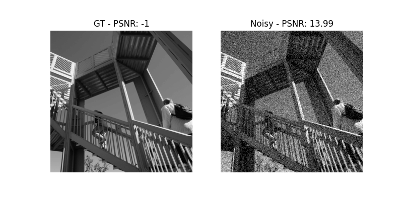
This example shows the denoising of an image with added normally distributed noise.

We create a scenario with a scaled demo image and add normally distributed noise with standard deviation of 0.2 is added.

import matplotlib.pyplot as plt
import numpy as np
from scipy import misc

from recon.utils.utils import psnr
from recon.interfaces import Smoothing, SmoothBregman

img = misc.ascent()
img = img/np.max(img)
gt = img

vmin, vmax = 0, 1

# create noisy image
sigma = 0.2 * vmax
n = np.random.normal(0, sigma, gt.shape)
noise_img = gt + n

f = plt.figure(figsize=(8, 4))
plt.gray()
f.add_subplot(1, 2, 1)
plt.title("GT - PSNR: "+str(psnr(gt, gt)))
plt.axis('off')
plt.imshow(gt, vmin=vmin, vmax=vmax)
f.add_subplot(1, 2, 2)
plt.gray()
plt.title("Noisy - PSNR: "+str(psnr(gt, noise_img)))
plt.imshow(noise_img, vmin=vmin, vmax=vmax)
plt.axis('off')
plt.show(block=False)

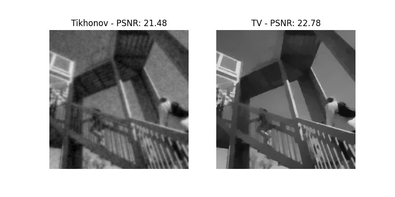
TV- and Tikhonov-Regularization. Basically, the problem here consists of two parts. The fidelity term and the regularization term. While we use the L2 norm to measure the proximity between the image and the degraded solution, the regularization term forces a low gradient-norm. In our case we distinguish between TV and Tikhonov. TV is called the L1-norm of the gradient, while Tikhonov represents the L2-norm. Overall, TV preserves edges better.

tv_smoothing = Smoothing(domain_shape=gt.shape, reg_mode='tv', lam=3, tau='calc')
u_tv = tv_smoothing.solve(data=noise_img, max_iter=3000, tol=1e-4)

tikh_smoothing = Smoothing(domain_shape=gt.shape, reg_mode='tikhonov', lam=0.1, tau='calc')
u_tik = tikh_smoothing.solve(data=noise_img, max_iter=3000, tol=1e-4)

f = plt.figure(figsize=(8, 4))
f.add_subplot(1, 2, 1)
plt.axis('off')
plt.gray()
plt.imshow(u_tik, vmin=vmin, vmax=vmax)
plt.title("Tikhonov - PSNR: "+str(psnr(gt, u_tik)))
f.add_subplot(1, 2, 2)
plt.imshow(u_tv, vmin=vmin, vmax=vmax)
plt.title("TV - PSNR: "+str(psnr(gt, u_tv)))
plt.axis('off')
plt.gray()
plt.show(block=False)

Out:

Early stopping.
Early stopping.

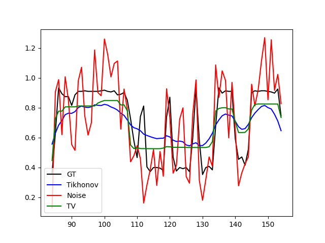
1D comparison with [gt, noise, Tikhonov, TV].

x_min = 84
x_max = 155
y = 20
plt.plot(range(x_min, x_max), gt[x_min:x_max,y], color="black", label="GT")
plt.plot(range(x_min, x_max), u_tik[x_min:x_max,y], color="blue", label="Tikhonov")
plt.plot(range(x_min, x_max), noise_img[x_min:x_max,y], color="red", label="Noise")
plt.plot(range(x_min, x_max), u_tv[x_min:x_max,y], color="green", label="TV")
plt.legend(loc="lower left")
plt.plot()
plt.show(block=False)

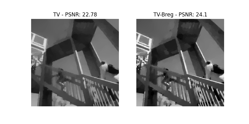
Bregman Iteration We start from an over-regularized solution and iterate through the degraded image with respect to the regularization functional (here TV). An emerging loss of contrast can thus be compensated.

breg_smoothing = SmoothBregman(domain_shape=gt.shape,
                               reg_mode='tv',
                               lam=1,
                               tau='calc',
                               plot_iteration=False,
                               assessment=sigma * np.sqrt(np.prod(gt.shape)))

u_breg = breg_smoothing.solve(data=noise_img, max_iter=2000, tol=1e-4)

f = plt.figure(figsize=(8, 4))
f.add_subplot(1, 2, 1)
plt.axis('off')
plt.gray()
plt.imshow(u_tv, vmin=vmin, vmax=vmax)
plt.title("TV - PSNR: "+str(psnr(gt, u_tv)))
f.add_subplot(1, 2, 2)
plt.imshow(u_breg, vmin=vmin, vmax=vmax)
plt.title("TV-Breg - PSNR: "+str(psnr(gt, u_breg)))
plt.axis('off')
plt.gray()
plt.show(block=False)

Out:

current norm error: 225.474801339
runs till norm <: 102.4
 Early stopping.
current norm error: 116.716062059
runs till norm <: 102.4
 Early stopping.
current norm error: 106.839905337
runs till norm <: 102.4
 Early stopping.
current norm error: 102.989571177
runs till norm <: 102.4
 Early stopping.

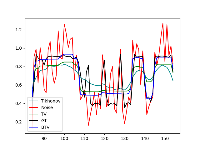
1d comparison with [gt, noise, BTV, TV, Tikhonov].

x_min = 84
x_max = 155
y = 20
plt.plot(range(x_min, x_max), u_tik[x_min:x_max,y], color="darkcyan", label="Tikhonov")
plt.plot(range(x_min, x_max), noise_img[x_min:x_max,y], color="red", label="Noise")
plt.plot(range(x_min, x_max), u_tv[x_min:x_max,y], color="green", label="TV")
plt.plot(range(x_min, x_max), gt[x_min:x_max,y], color="black", label="GT")
plt.plot(range(x_min, x_max), u_breg[x_min:x_max,y], color="blue", label="BTV")
plt.legend(loc="lower left")
plt.show(block=False)